Line Profiles
It can be useful to look at a line profile, for example in the height
data. You can use AFM.lineProfile() to get an arbitrary
line, or AFM.getLine(), if you want to select a horizontal
line. In the example below, we provide the coordinates in units of [nm],
however, you can also provide the coordinates in pixels, if you set
unitPixels to TRUE. Alternatively, if you are
not providing any coordinates, you can click on two points to select a
profile line.
library(ggplot2)
library(scales)
filename = AFM.getSampleImages(type='tiff')
afmd = AFM.import(filename)
# afmd2 = AFM.lineProfile(afmd)  # click on two points on the image
afmd2 = AFM.lineProfile(afmd, 200,2050, 800,2050, verbose = TRUE)
#> [1] "Pixels: ( 21 , 210 ) - ( 81 , 209 )"
#> delta Y: 9.804 nm/px and delta X: 9.804 nm/px
afmd2 = AFM.lineProfile(afmd2, 200,2080, 800,2080)

plot(afmd2, addLines = TRUE, trimPeaks = 0.01)
#> Graphing: Topography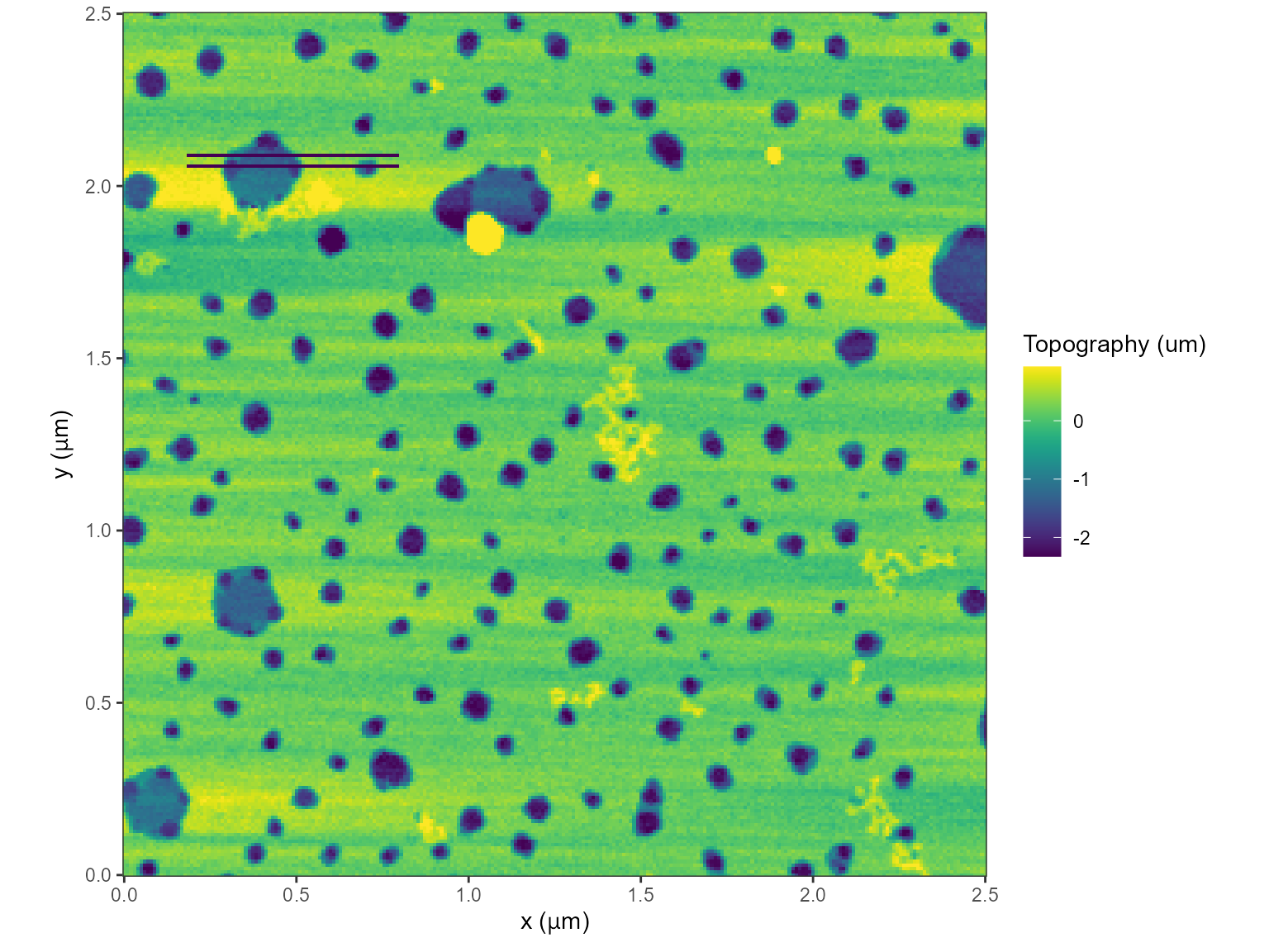
This shows where the profile line is measured; the units are in
nm, according to the AFM image.
AFM.linePlot(afmd2)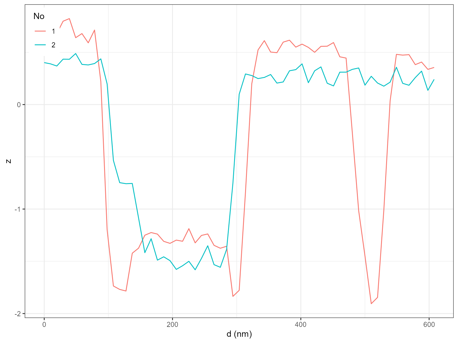
dLine = AFM.linePlot(afmd2, dataOnly = TRUE)
head(dLine)
#>           x         z type
#> 1  0.000000 0.8030308    1
#> 2  9.803922 0.6511638    1
#> 3 19.607843 0.7997923    1
#> 4 29.411765 0.8113265    1
#> 5 39.215686 0.7050135    1
#> 6 49.019608 0.6748323    1
The line plot has a lowest point at -1.83 nm, and a maximum at 0.811 nm.