library(nanoAFMr)
#> Please cite nanoAFMr 2.1.11 , see https://doi.org/10.5281/zenodo.7464877
library(ggplot2)
library(scales)
filename = AFM.getSampleImages(type='tiff')
afmd = AFM.import(filename)
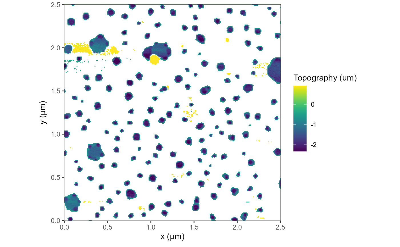
plot(afmd)
#> Graphing: Topography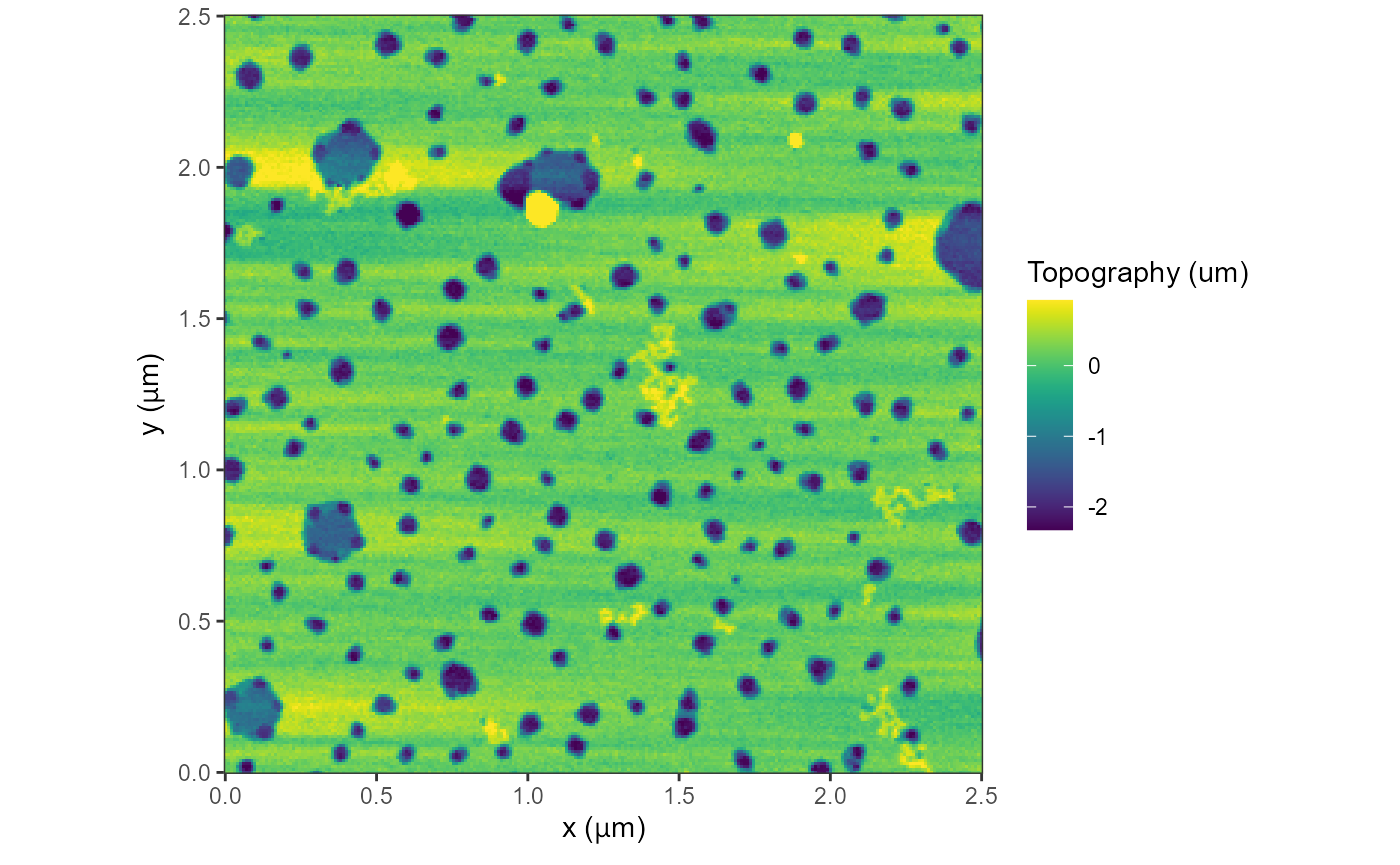
In order to get more contrast, we can trim 1 percent of the data points as the image may not be in the middle, see the histogram.
AFM.histogram(afmd)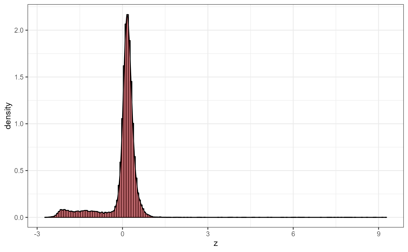
Using the trimPeaks option in plot(), we
can remove half from the top and bottom of the histogram and bunch those
data points up, so that the contrast enhances.
plot(afmd, trimPeaks = 0.01)
#> Graphing: Topography
Raster Graph
Graphing a subset of the data points using the
AFM.raster() function to obtain the 3D data point set.
dr = AFM.raster(afmd)
head(dr)
#>           x y          z
#> 1  0.000000 0  0.1887319
#> 2  9.803922 0  0.2422829
#> 3 19.607843 0  0.3089453
#> 4 29.411765 0  0.1487159
#> 5 39.215686 0 -0.1791730
#> 6 49.019608 0 -0.7145596
# data points higher than 90% of peak
lowerBound = -0.3
upperBound = 0.8
dr1 =dr[which(dr$z>lowerBound & dr$z<upperBound),]
plot(afmd, trimPeaks = 0.01) +
  geom_raster(data=dr1,fill='white')
#> Graphing: Topography