library(nanoAFMr)
#> Please cite nanoAFMr 2.1.11 , see https://doi.org/10.5281/zenodo.7464877
library(ggplot2)
The Height-Height Correlation Function is discussed in the publication: Height-Height Correlation Function to Determine Grain Size in Iron Phthalocyanine Thin Films Thomas Gredig, Evan A. Silverstein, Matthew P Byrne, Journal: J of Phys: Conf. Ser. Vol 417, p. 012069 (2013).
It defines a correlation function \(g(r)\) as follows:
\[ g(r) = <| (h(\vec{x}) - h(\vec{x}-\vec{r}) |^2 > \]
where \(h(\vec{x})\) is the height at a particular location. The height difference is computed for all possible height pairs that are separated by a distance \(|\vec{r}|\). Immediately, if follows that \(g(0)=0\).
For a set of images, the correlation function can be interpreted as follows:
\[ g'(r) = 2\sigma^2 \left[ 1- e^{- \left(\frac{r}{\xi}\right)^{2\alpha}} \right] \]
which has 3 fitting parameters, the long-range roughness \(\sigma\), the short-range roughness \(\alpha\) (Hurst parameter), and the correlation length \(\xi\).
Example: HHCF
The computation is implemented in this package as follows, the image
is flattened, then HHCF is computed and the curve is fit. Choosing a
large number of iterations is crucial. The computation is executed with
the AFM.hhcf() function.
filename = AFM.getSampleImages(type='tiff')
a = AFM.import(filename)
a = AFM.flatten(a)
AFM.hhcf(a, numIterations= 2e5)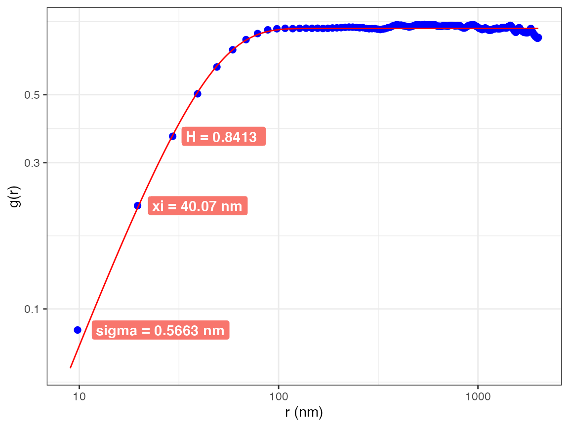
You can see the fit parameters, and make a custom plot from the data, if you export all results from the function
library(pander)
h = AFM.hhcf(a, numIterations= 2e5, allResults = TRUE)

## show the fit parameters
pander(h$fitParams)| sigma | xi | Hurst | sigma.err | xi.err | Hurst.err |
|---|---|---|---|---|---|
| 0.6434 | 40.74 | 0.8432 | 0.0004259 | 0.5936 | 0.02996 |
## show the HHCF data
head(h$data)
#> r.nm g num
#> 1 9.803922 0.08386283 199522
#> 2 19.607843 0.21302400 198641
#> 3 29.411765 0.36214199 197691
#> 4 39.215686 0.49741077 196759
#> 5 49.019608 0.61137055 195779
#> 6 58.823529 0.69628173 194790
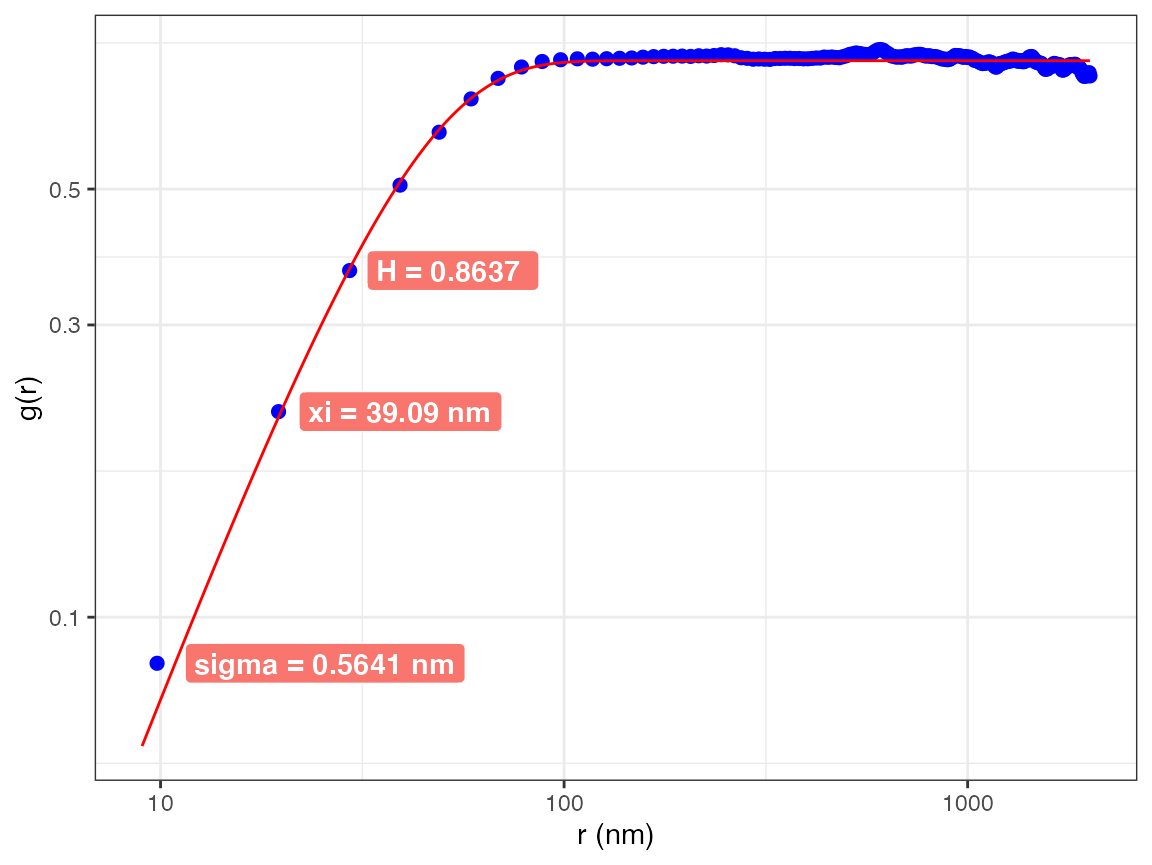
## display the entire graph
h$graph