Find all the frequency sweep files:
library(nanoAFMr)
filesAFM = AFM.getSampleImages()
freqAFM = filesAFM[sapply(filesAFM, function(x) { (AFM.dataType(AFM.import(x)) == 'frequency') })]
Frequency Sweep Graph
You can import the frequency file as an AFMdata file
using the standard import function. Graphing also works with the
plot.AFMdata() function.
a = AFM.import(freqAFM[1])
plot(a)
#> Graphing: Frequency sweep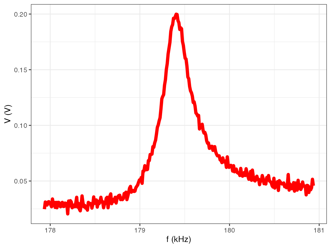
Frequency Sweep Info
print(a)
#> Object      : NanoSurf AFM frequency
#> Description : Aspire CT170R-25; 179.405kHz; 284mV; 15-02-2012; 21:23:59
#> Channel     : Frequency sweep
#> Resolution  : 177935 Hz  -  180935 Hz
#> History     :
#> Filename    : /private/var/folders/bz/zk25f6614w5b3_f61czs2dtc0000gr/T/Rtmp3VmG9r/temp_libpath12ca60a44957/nanoAFMr/extdata/NanoSurf_resonancePeak.nid
summary(a)
#>            objectect                                               description
#> 1 NanoSurf frequency Aspire CT170R-25; 179.405kHz; 284mV; 15-02-2012; 21:23:59
#>   resolution            size         channel history z.min  z.max z.units
#> 1        301 177935 - 180935 Frequency sweep           148 179405      Hz
#>    dataType
#> 1 frequency
Frequency Sweep Data
You can extract the data from the graph using the
AFM.raster() function:
d = AFM.raster(a)
head(d)
#>   freq.Hz        z.V
#> 1  177935 0.02471924
#> 2  177945 0.03112793
#> 3  177955 0.02899170
#> 4  177965 0.02838135
#> 5  177975 0.03112793
#> 6  177985 0.03143311