Force versus Distance Curves
This example illustrates how to extract force versus distance spectroscopy data from Park AFM images:
f = AFM.getSampleImages('force')
a = AFM.import(f)
a = AFM.flatten(a)
plot(a) + labs(fill="z (nm)")
#> Graphing: Topography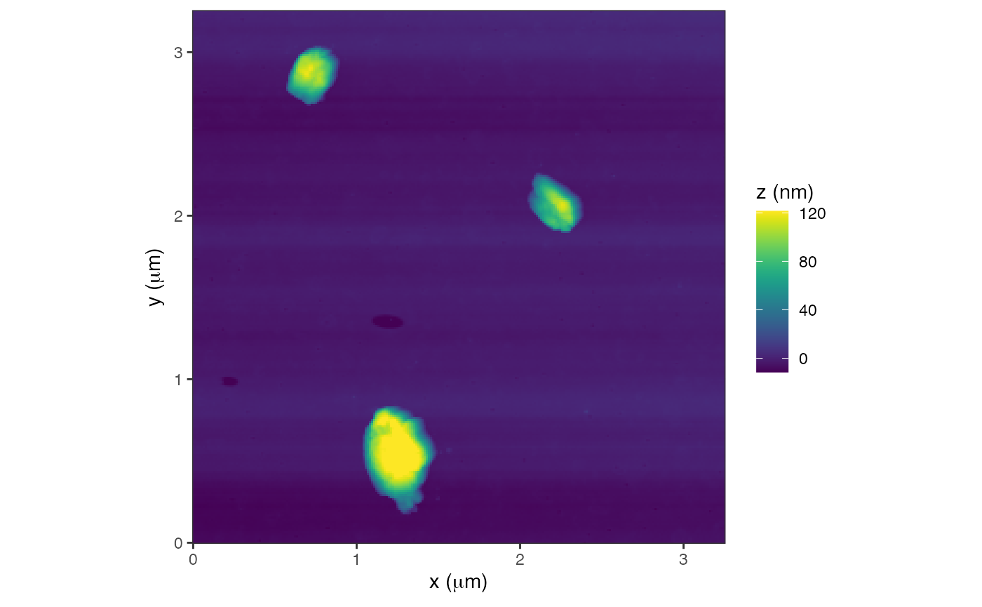
Spectroscopy data files are recognized as such:
AFM.dataType(a)
#> [1] "spectroscopy"
The file can be graphed like a regular AFM file, but additionally, it contains the spectroscopy data. Several channels are recorded:
AFM.specHeader(a)
#> channelName channelUnit channelGain channelXaxis channelYaxis offset
#> 1 Vertical (A-B) V 1 0 1 0
#> 2 Force nN 1 0 1 0
#> 3 Z Scan um 1 1 0 0
#> 4 Z Detector um 1 1 0 0
#> 5 Time Stamp usec 1 1 0 0
#> 6 1 0 0 0
#> 7 1 0 0 0
#> 8 1 0 0 0
#> logScale square
#> 1 0 0
#> 2 0 0
#> 3 0 0
#> 4 0 0
#> 5 0 0
#> 6 0 1
#> 7 0 0
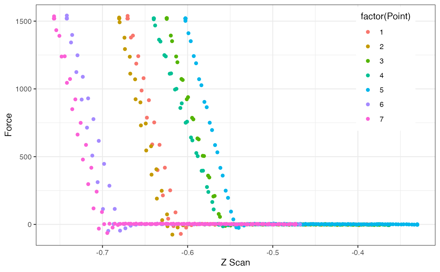
#> 8 0 -1074790400The data from these channels is extracted as follows:
df = AFM.specData(a)
ggplot(df, aes(`Z Scan`, Force, col=factor(Point))) +
  geom_point() +
  theme_bw() +
  theme(legend.position = c(0.95,0.99),
        legend.justification = c(1,1))