Loading AFM image
fname = AFM.getSampleImages()[1]
afmd = AFM.import(fname)
The AFM image can be displayed using graphTypes:
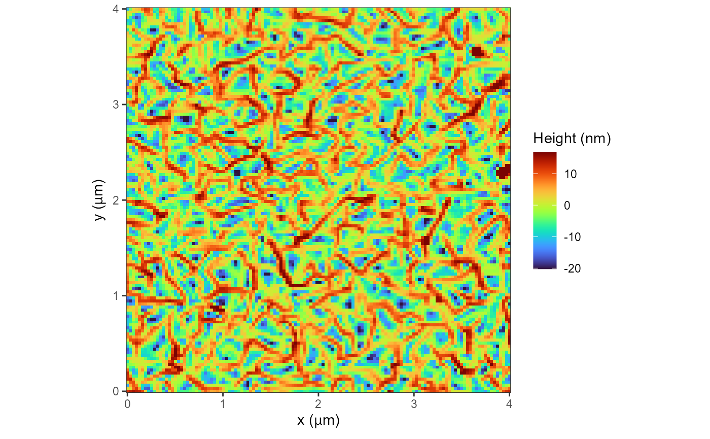
graphType 1
This is the basic and default graph for an AFM image:
q = plot(afmd, graphType=1, trimPeaks=0.01)
#> Graphing: HeightRetrace
graphType 2
This graph has a square shape and adds a bar of length 20%; it places the scale inside the graph.
plot(afmd, graphType=2,trimPeaks=0.01)
#> Graphing: HeightRetrace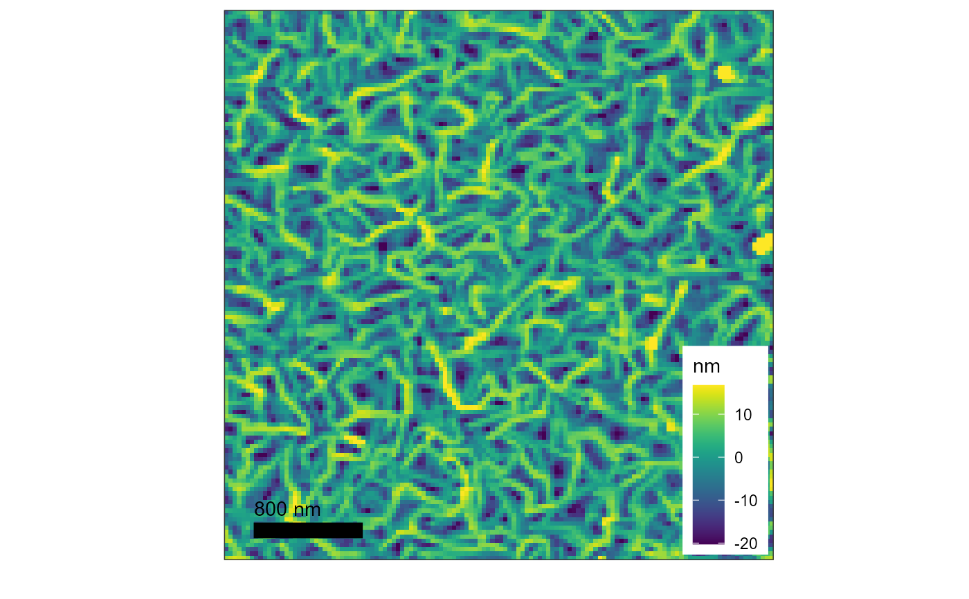
The image can be saved with ggsave as it is graphed with
ggplot.
graphType 3
This graph type is bare and has neither length scales nor legend.
plot(afmd, graphType=3, trimPeaks=0.01)
#> Graphing: HeightRetrace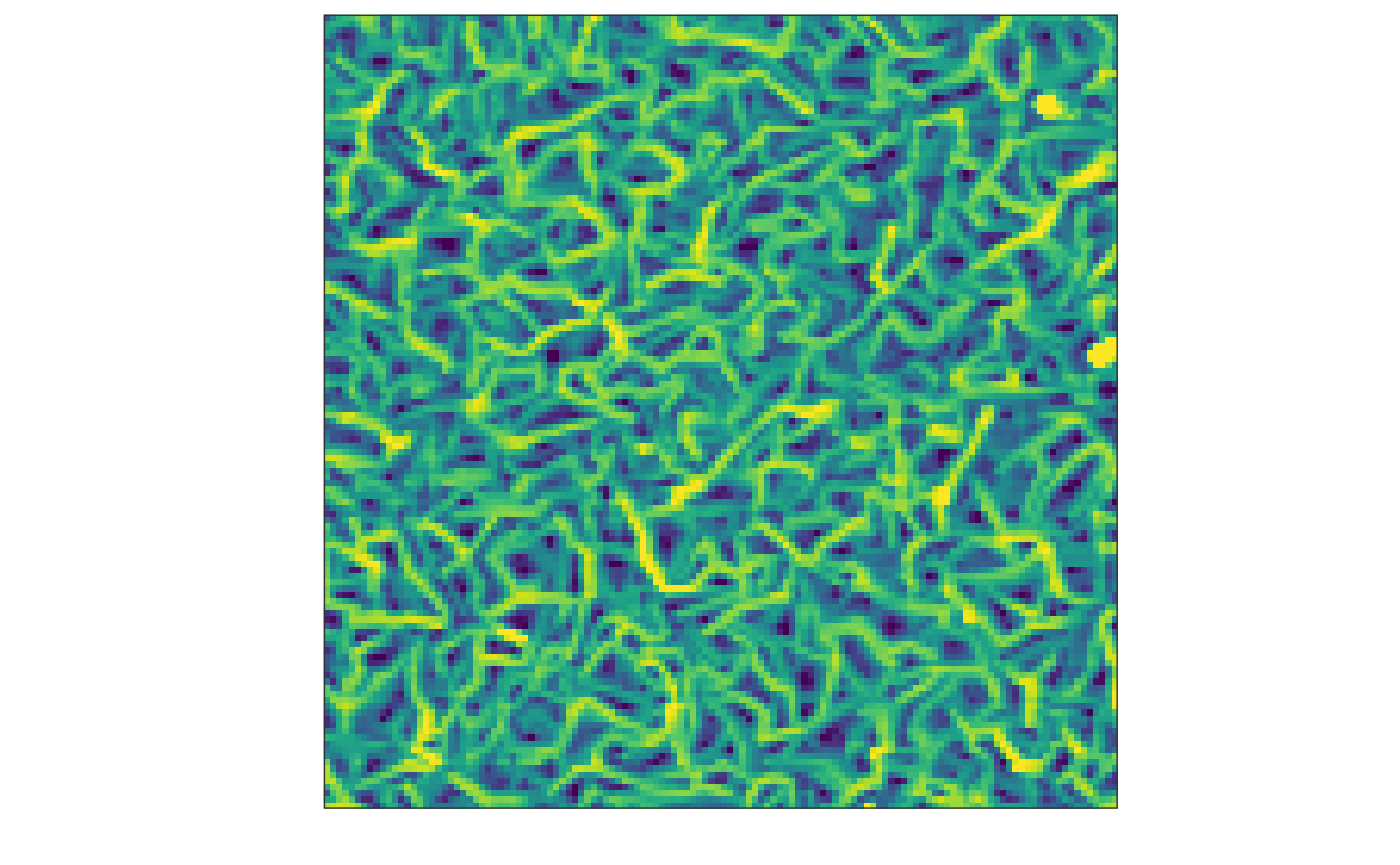
summary(afmd)
#>      objectect               description resolution           size
#> 1 Cypher image KC200, FePc, KC20170720Si  128 x 128 4000 x 4000 nm
#> 2 Cypher image KC200, FePc, KC20170720Si  128 x 128 4000 x 4000 nm
#> 3 Cypher image KC200, FePc, KC20170720Si  128 x 128 4000 x 4000 nm
#> 4 Cypher image KC200, FePc, KC20170720Si  128 x 128 4000 x 4000 nm
#>            channel history     z.min    z.max z.units dataType
#> 1    HeightRetrace         -32.45992 50.78832      nm    image
#> 2 AmplitudeRetrace          29.00730 32.78488      nm    image
#> 3     PhaseRetrace          63.92822 85.18923     deg    image
#> 4   ZSensorRetrace         -29.44336 48.16414      nm    image
graphType 4
This graph type is plain with a scale. You can also change the color and the size of the font that displays the scale.
plot(afmd, graphType=4, col='white', size=10, trimPeaks=0.05, fillOption = 'A')
#> Graphing: HeightRetrace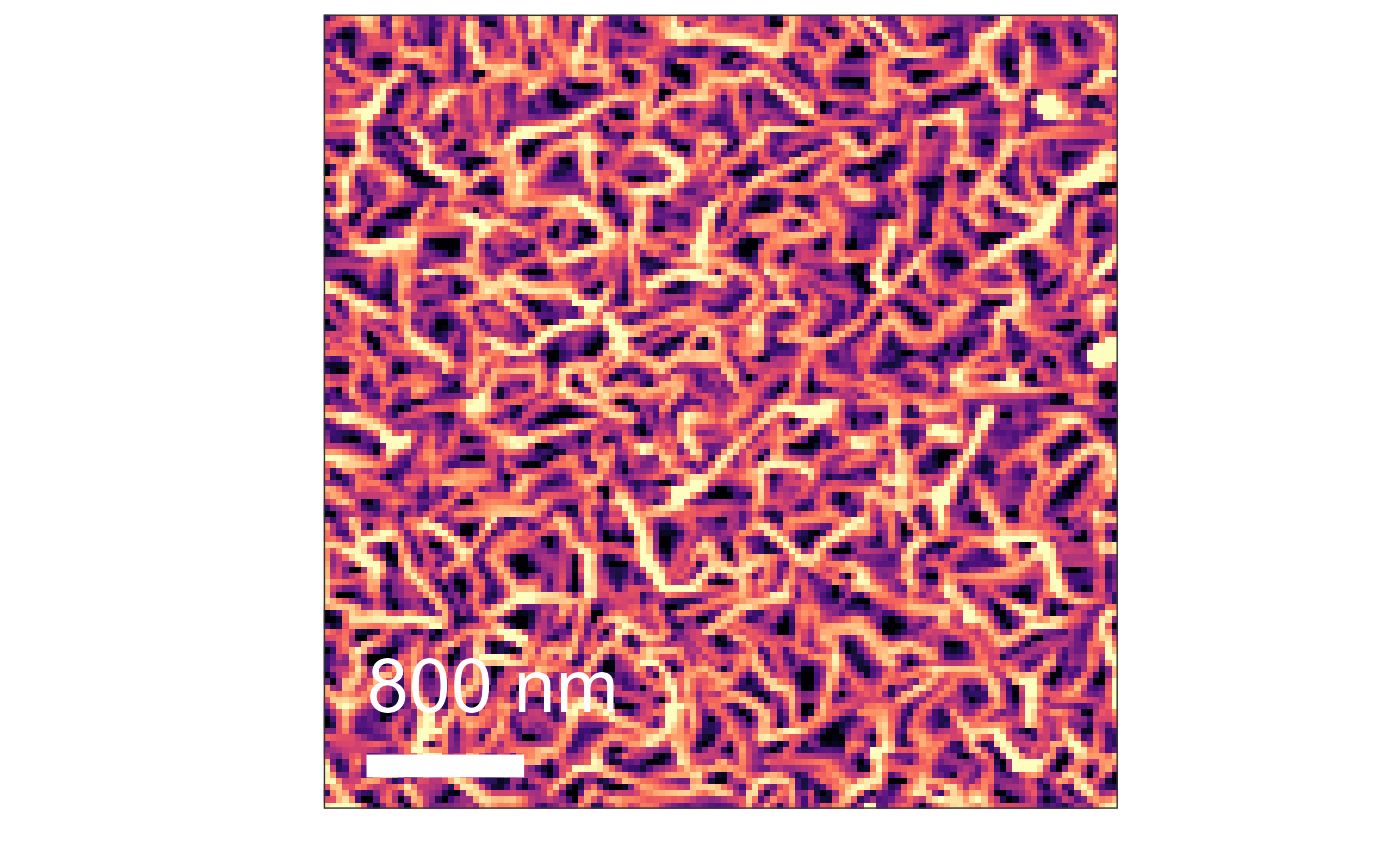
Red Blue Color Scheme
This graph type is bare and has neither length scales nor legend.
plot(afmd, graphType=1, trimPeaks=0.01, redBlue = TRUE)
#> Graphing: HeightRetrace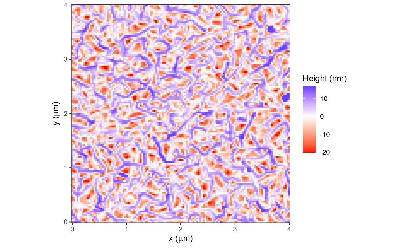
Graphing 2 plots side by side
Use the package cowplot to create a graph with two
plots. Use save_plot to save the graph.
library(cowplot)
library(latex2exp)
fname2 = AFM.getSampleImages(type='ibw')[1]
afmd = AFM.import(fname2)

g1 = plot(afmd, trimPeaks=0.01, graphType = 1) +
  labs(fill='h (nm)') + theme(legend.key.size = unit(1, 'char'))
#> Graphing: HeightRetrace
g2 = plot(afmd, no=2, trimPeaks=0.01, graphType = 1, mpt=29.6) +
  labs(fill="A (nm)") + theme(legend.key.size = unit(1, 'char'))
#> Graphing: AmplitudeRetrace
g3 = plot(afmd, no=3, trimPeaks=0.01, graphType = 1, mpt=65.5) +
  labs(fill=TeX("$\\phi$ (deg)")) + theme(legend.key.size = unit(1, 'char'))
#> Graphing: PhaseRetrace
g4 = plot(afmd, no=4, trimPeaks=0.01, graphType = 1) +
  labs(fill="z (nm)") + theme(legend.key.size = unit(1, 'char'))
#> Graphing: ZSensorRetrace
gAll = plot_grid(g1, g2, g3, g4,
          labels=c('a','b','c','d'))
ggdraw(add_sub(gAll,
               "Showing surface morphology of a phthalocyanine thin film\n with (a) height h, (b) amplitude A, (c) phase ϕ, and \n (d) z-sensor z response. Sample / image from Gredig\n Lab, CSU Long Beach.",
               x=0.1, hjust=0))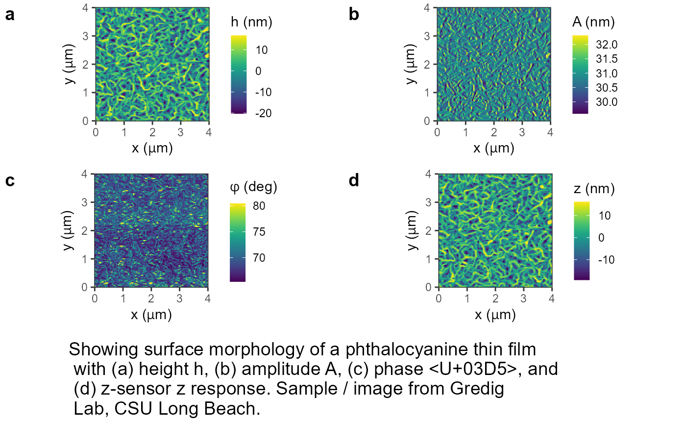
Changing the Color Palette
You can use the fillOption option to change the color
palette, see also ? scale_fill_viridis. There are 8
options:
plot(afmd, graphType = 1, fillOption = "magma")
#> Graphing: HeightRetrace
plot(afmd, graphType = 1, fillOption = "inferno")
#> Graphing: HeightRetrace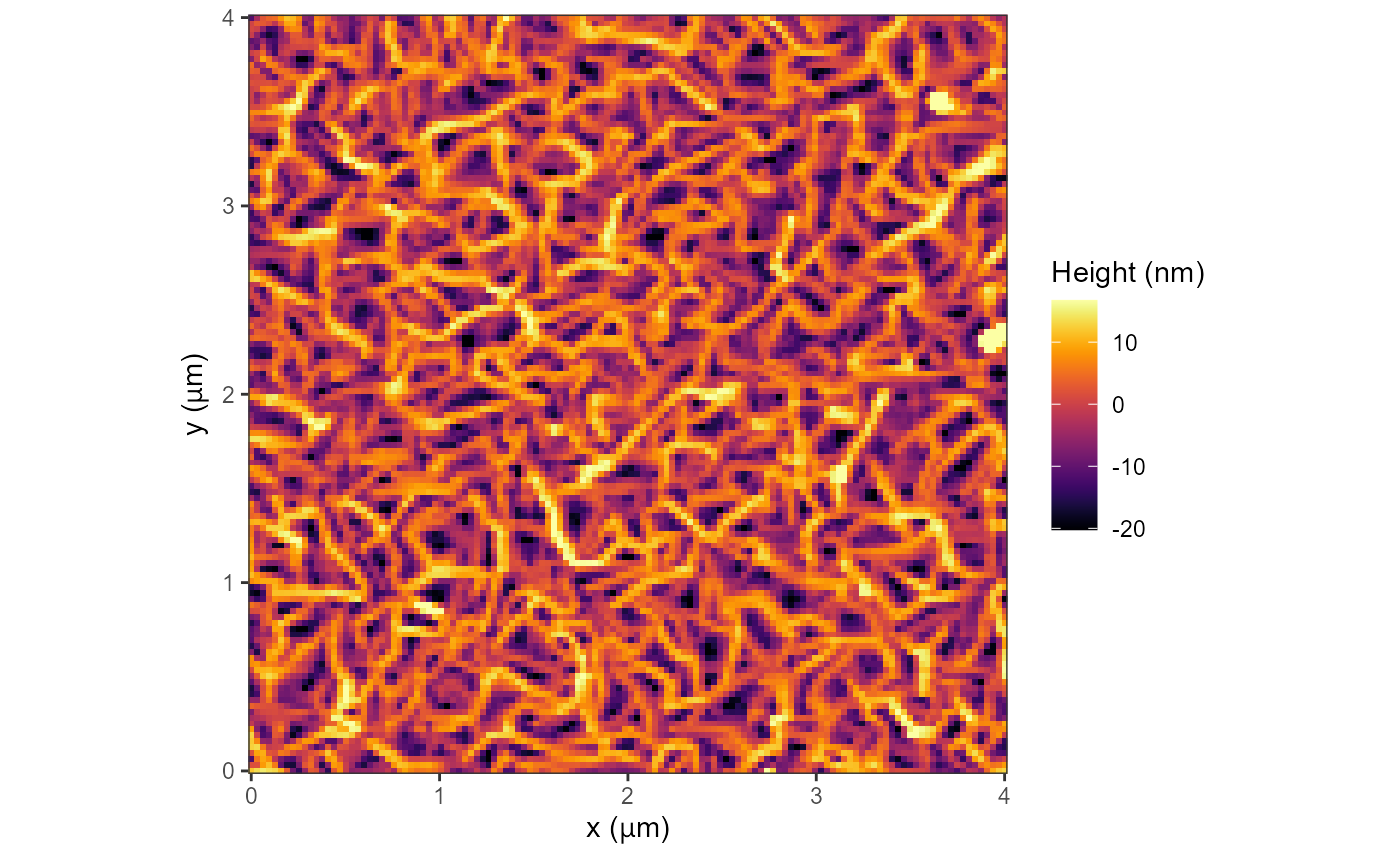
plot(afmd, graphType = 1, fillOption = "plasma")
#> Graphing: HeightRetrace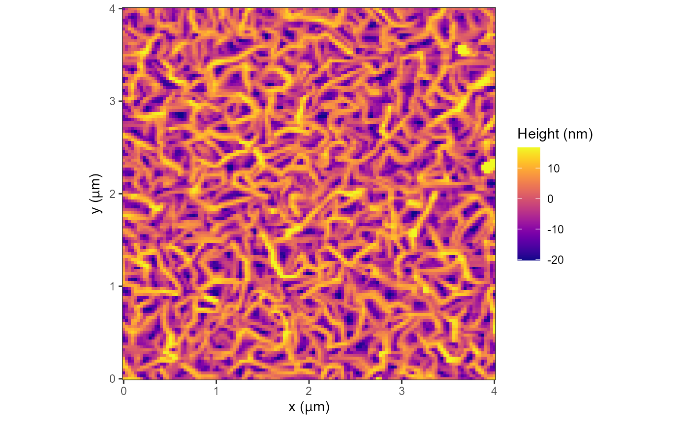
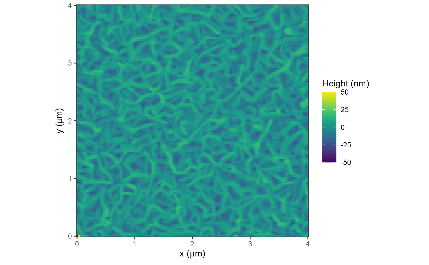
plot(afmd, graphType = 1, fillOption = "viridis")
#> Graphing: HeightRetrace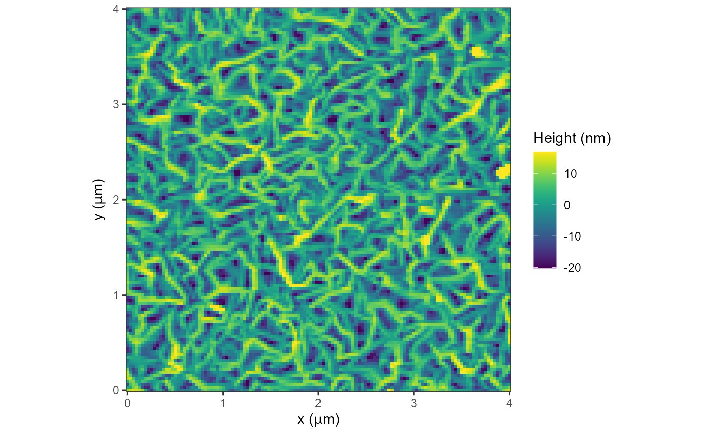
plot(afmd, graphType = 1, fillOption = "cividis")
#> Graphing: HeightRetrace
plot(afmd, graphType = 1, fillOption = "rocket")
#> Graphing: HeightRetrace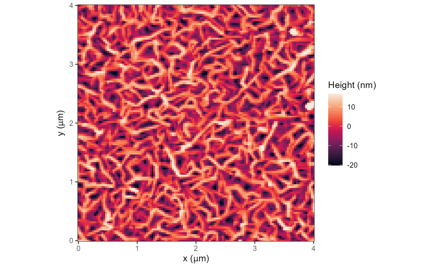
plot(afmd, graphType = 1, fillOption = "mako")
#> Graphing: HeightRetrace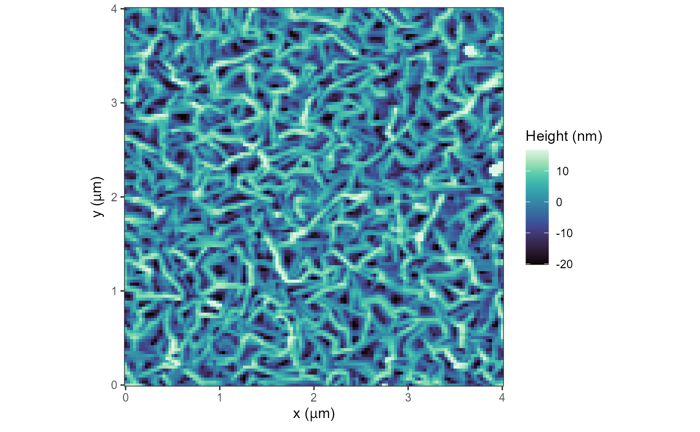
plot(afmd, graphType = 1, fillOption = "turbo")
#> Graphing: HeightRetrace