Line Profile

create a profile data line across an image (d), providing the starting point (x1,y1) and end point (x2,y2). The start and end points are provided in units of nanometers or pixels. If the starting and end point coordinates are not provided, it will use the raster::click() function to prompt the user to click on two points on the graph.

Note: the convention is that the bottom left corner is (1,1) in pixels and (0,0) in nanometers

AFM.lineProfile(
  obj,
  x1 = NA,
  y1 = NA,
  x2 = NA,
  y2 = NA,
  N = 1,
  unitPixels = FALSE,
  verbose = FALSE
)

Arguments

obj

AFMdata object

x1

start x position in units of nm/pixels from bottom left, if NA, user will need to click on two points to define profile line

y1

start y position in units of nm/pixels from bottom left, if NA, user will need to click on two points to define profile line

x2

end x position in units of nm/pixels from bottom left, if NA, user will need to click on two points to define profile line

y2

end y position in units of nm/pixels from bottom left, if NA, user will need to click on two points to define profile line

N

thickness of line in pixels, for high-resolution images, increase

unitPixels

logical, if TRUE, then coordinates are in units of pixels otherwise nm

verbose

logical, if TRUE, output additional information

Value

AFMdata object with line data, use AFM.linePlot() to graph / tabulate data or plot(addLines=TRUE) to graph image with lines

See also

[AFM.getLine(), AFM.liniePlot(), plot.AFMdata()]

Author

Thomas Gredig

Examples

afmd = AFM.artificialImage(width=128, height=128, type='calibration', verbose=FALSE)
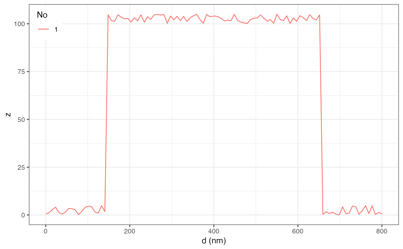
AFM.lineProfile(afmd, 100, 500, 900, 500) -> afmd2
AFM.linePlot(afmd2)


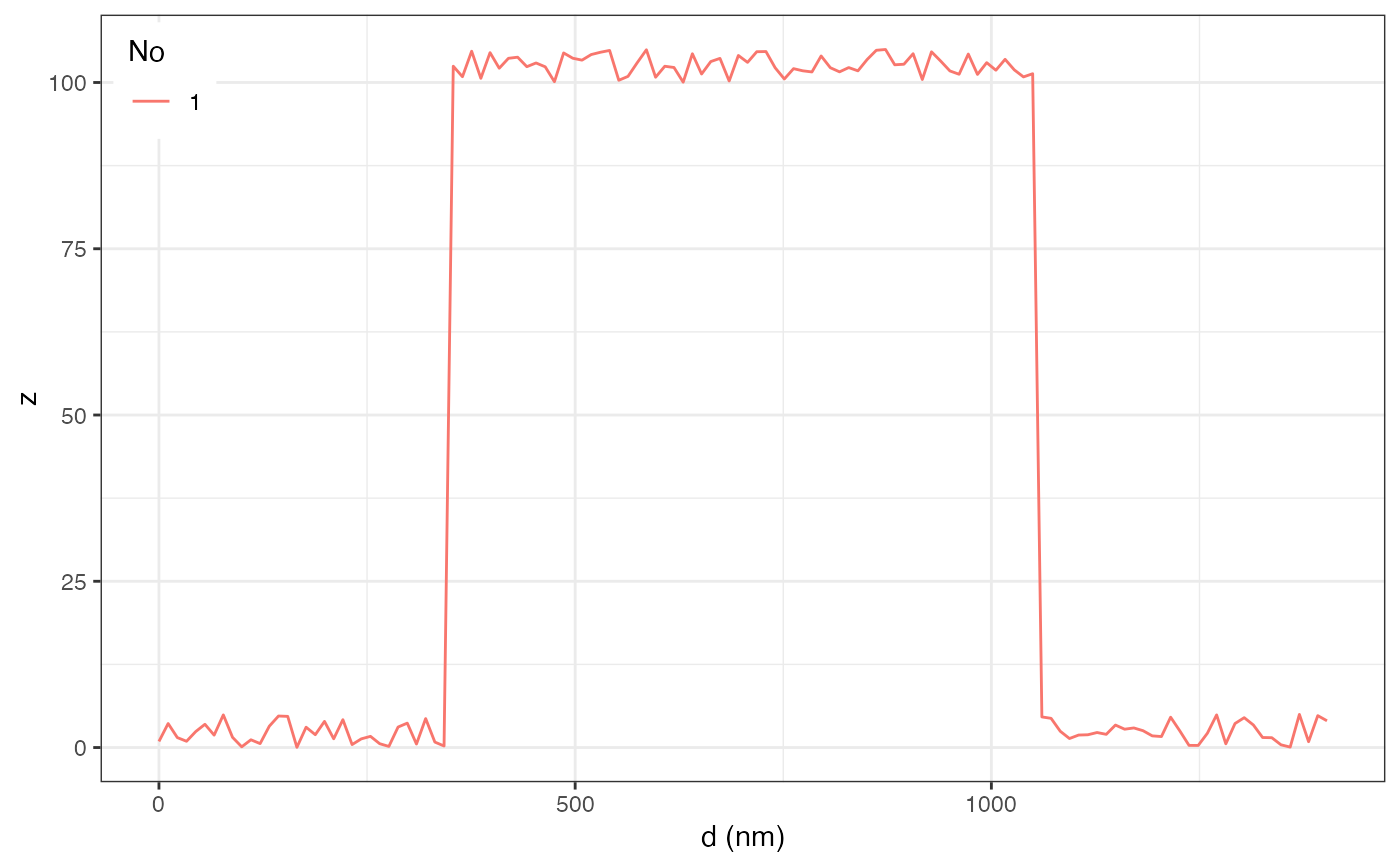
AFM.lineProfile(afmd, 1, 1, 128, 128, unitPixels=TRUE) -> afmd2
AFM.linePlot(afmd2)

head(AFM.linePlot(afmd2, dataOnly=TRUE))
#>          x         z type
#> 1  0.00000 0.9193581    1
#> 2 11.04854 3.6079403    1
#> 3 22.09709 1.4946407    1
#> 4 33.14563 0.9417131    1
#> 5 44.19417 2.4014746    1
#> 6 55.24272 3.4955050    1