Coercivity
Coercivity.Rmd
library(quantumPPMS)No diamagnetic correction
The coercivity can be estimated from the versus curves. Here is an example to retrieve the coercive field values; note that in this example, the diamagnetic background has not been removed, so the result should be interpreted accordingly
filename = vsm.getSampleFiles()[1]
d = vsm.import(filename)
d1 = vsm.getLoop(d, lp=1, direction=1 )
df = vsm.data.frame(d1)
Hc = vsm.get.Coercivity(df$H, df$M)
print(paste("Coercivity is ", signif(Hc,3),"Oe."))
#> [1] "Coercivity is  428 Oe."
Let us check whether the value agrees visually:
plot(d1)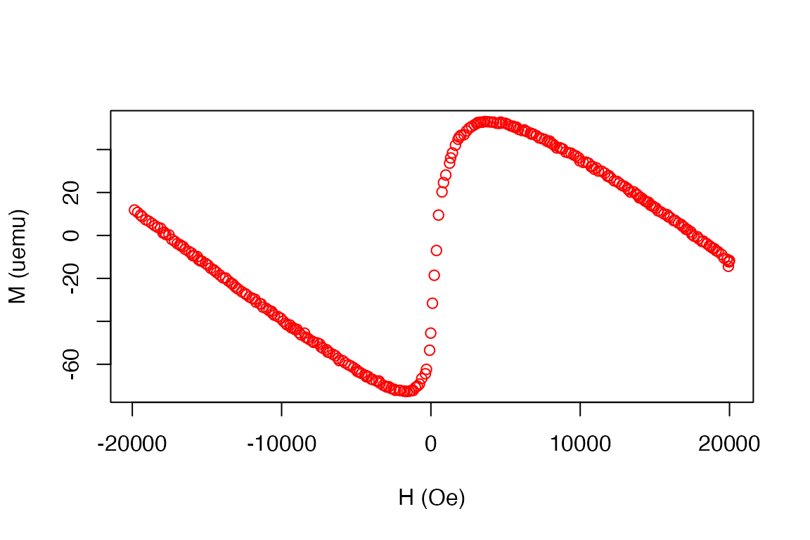
plot(df$H, df$M, xlim=c(-(2*Hc),+(2*Hc)), pch=19, col='blue')
lines(df$H, df$M)
abline(h = 0, v=Hc, col='red')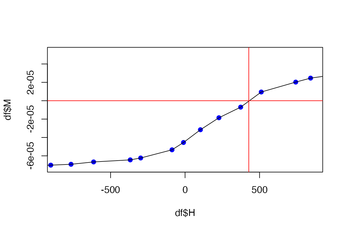
With diamagnetic correction
filename = vsm.getSampleFiles()[1]
d = vsm.import(filename)
dStats = vsm.hystStats(d)
t(dStats)
#>                   [,1]            [,2]
#> H.first           "-19852.77"     " 20000.26"
#> H.last            " 19999.11"     "-19999.97"
#> H.max             "19999.11"      "20000.26"
#> H.min             "-19852.77"     "-19999.97"
#> Ms1               "8.630711e-05"  "9.373929e-05"
#> Ms1.sd            "3.463391e-07"  "3.372475e-07"
#> Ms2               "-8.633927e-05" "-9.198534e-05"
#> Ms2.sd            "5.919962e-07"  "4.418546e-07"
#> Hc                " 413.6"        "-453.2"
#> Hc.err            "76.4"          "80.4"
#> Hc.nFit           "7"             "7"
#> Mrem              "-3.901093e-05" " 4.013892e-05"
#> Mrem.sd           "1.778054e-06"  "2.604337e-06"
#> Susceptibility    "-4.879e-09"    "-5.265e-09"
#> Susceptibility.sd "3.171e-11"     "3.945e-11"
#> T                 "2.999695"      "3.000080"
#> T.sd              "0.001849705"   "0.001832903"
#> speed             " 104.4547"     "-104.1414"
#> speed.sd          "0.09317400"    "0.09936709"
#> time.delta        "397.88"        "412.13"
#> data.points       "263"           "257"
#> dir               " 1"            "-1"
#> type              "MvsH"          "MvsH"
#> loop              "1"             "1"
print(paste("Coercivity is ", signif(dStats$Hc,3),"Oe."))
#> [1] "Coercivity is  414 Oe."  "Coercivity is  -453 Oe."
Hc = dStats$Hc
Let us check whether the value agrees visually:
df = vsm.data.frame(d)
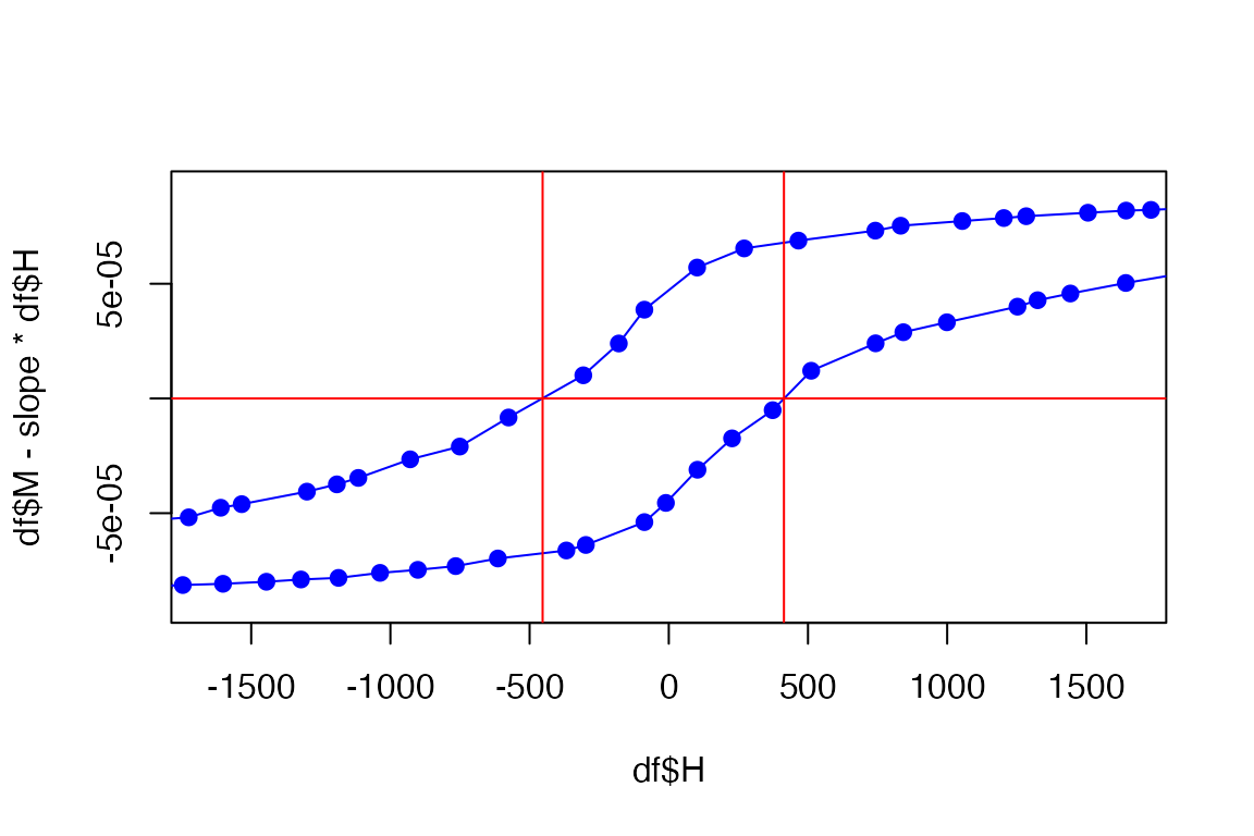
mean(dStats$Susceptibility) -> slope
plot(df$H, df$M - slope*df$H)
lines(df$H, df$M)
plot(df$H, df$M - slope*df$H, xlim=c(-(4*Hc[1]),+(4*Hc[1])), pch=19, col='blue')
lines(df$H, df$M  - slope*df$H, col='blue')
abline(h = 0, v=Hc, col='red')